1
2
3
4
import numpy as np
import pandas as pd
from IPython.core.interactiveshell import InteractiveShell
InteractiveShell.ast_node_interactivity = "all"
https://scikit-learn.org/stable/modules/cross_validation.html#cross-validation-iterators
1.교차검증
기본적으로 데이터는 train data 와 test data로 나누어서 학습을 진행한다
이때, test data는 반드시 한번만 사용한다
하지만 단순히 train 과 test data로 분리하는것 만으로 충분하지 않다 => overfitting 취약하다
why? => train + test만을 가지고 학습과 평가를 하면 결국 모델은 고정된 test set에만 과적합는 모델이 만들어진다. 이로 인해 다른 unseen data에는 성능이 떨어진다
교차검증: test data를 제외하고 별도의 여러 세트로 구성된 train 과 validation data를 학습과 평가를 위해 사용한다
<Ultimate Scheme>
전체 데이터 train_test_split 으로 나눈다
train_set만을 가지고 교차검증 진행
교차검증을 통한 최종 모델 선택
마지막으로 test_set으로 평가
2.교차검증의 종류
여러 종류가 존재한다 => 때에 따라 적절한 종류를 선택하는것이 아주중요하다
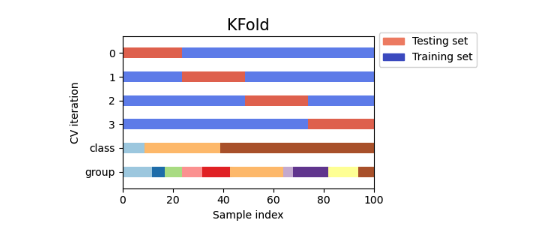
Kfold : 가장 일반적인 교차검증 방식
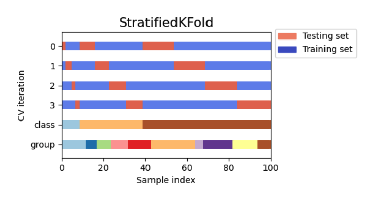
Stratified Kfold : for imbalanced
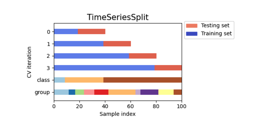
TimeSeriesSplit: 의미있는 시간적 순서를 갖는 데이터가 존재할때
그 외에도 다양한 방법 존재한다, 위에 url 참고하자
각 교차범증 방법 비교에 앞써서 데이터 준비하자
1
2
3
4
5
6
7
8
9
10
from sklearn.datasets import load_iris
from sklearn.tree import DecisionTreeClassifier
from sklearn.metrics import accuracy_score
from sklearn.model_selection import KFold
iris = load_iris()
features = iris.data
target = iris.target
iris_df = pd.DataFrame(features,columns=iris.feature_names)
iris_df['label'] = target
dt_clf = DecisionTreeClassifier(random_state=156)
3.KFold
쉡게 말해 데이터 셋을 n 개의 집단으로 구분
n-1개의 잡단을 train set, 1개의 집단을 validation set 으로 사용
총 n번의 학습과 평가가 이루어진다
이때, validation set을 순차적으로 사용해서 모두 다른 validation set으로 평가가 가능해진다
1
2
3
4
5
6
7
8
9
10
11
# 사용 방법을 먼저 알아보자

# Kfold 선언
kfold = KFold(n_splits=5) # shuffle은 defulat:false 다

# Kfold 의 split() 호출하면 train, val 데이터의 row index를 return한다

for train_index , test_index in kfold.split(features):
    test_index

# 아래의 결과를 보면 validation set 을 위한 row index들이 겹치는거 없이 순차적으로 5개 나오는거 확인할수 있다
array([ 0,  1,  2,  3,  4,  5,  6,  7,  8,  9, 10, 11, 12, 13, 14, 15, 16,
       17, 18, 19, 20, 21, 22, 23, 24, 25, 26, 27, 28, 29])
array([30, 31, 32, 33, 34, 35, 36, 37, 38, 39, 40, 41, 42, 43, 44, 45, 46,
       47, 48, 49, 50, 51, 52, 53, 54, 55, 56, 57, 58, 59])
array([60, 61, 62, 63, 64, 65, 66, 67, 68, 69, 70, 71, 72, 73, 74, 75, 76,
       77, 78, 79, 80, 81, 82, 83, 84, 85, 86, 87, 88, 89])
array([ 90,  91,  92,  93,  94,  95,  96,  97,  98,  99, 100, 101, 102,
       103, 104, 105, 106, 107, 108, 109, 110, 111, 112, 113, 114, 115,
       116, 117, 118, 119])
array([120, 121, 122, 123, 124, 125, 126, 127, 128, 129, 130, 131, 132,
       133, 134, 135, 136, 137, 138, 139, 140, 141, 142, 143, 144, 145,
       146, 147, 148, 149])
Shuffle
일단 shuffle을 한다는건 데이터가 특정 temproal ordering 에 상관이 없다는거다.
temporal ordering이 중요하면 섞으면 안된다.
또한, shuffle 을 한다고 해서 무조건 성능이 올라가는건 아니다.
Kfold에서 shuffle을 하게 되면 일단 먼저 데이터를 shuffle 한 후에 split이 진행되는거다. \
Shuffle 이후의 방식은 기본의 Kfold에서의 split 하는 방식이랑 정확하게 동일하다. (순차적으로 set을 만들어서 진행)
1
2
3
4
5
6
7
# shuffle
kfold = KFold(n_splits=5,shuffle=True)

# Kfold 의 split() 호출하면 train, val 데이터의 row index를 return한다

for train_index , test_index in kfold.split(features):
    test_index
array([  1,   8,   9,  14,  25,  27,  28,  34,  35,  39,  40,  43,  46,
        50,  62,  67,  69,  70,  71,  79,  83,  86,  89, 103, 104, 112,
       119, 126, 144, 149])
array([  0,   3,   6,  13,  22,  30,  31,  37,  49,  51,  56,  74,  88,
        91,  92,  94,  99, 107, 110, 113, 116, 121, 122, 127, 129, 130,
       133, 138, 143, 147])
array([  2,   5,  10,  12,  18,  20,  24,  32,  36,  52,  54,  57,  58,
        65,  66,  68,  77,  82,  84,  95,  97, 108, 114, 117, 118, 125,
       132, 135, 146, 148])
array([  7,  11,  21,  23,  26,  33,  38,  41,  45,  48,  55,  60,  61,
        64,  73,  75,  81,  90,  98, 101, 102, 105, 115, 134, 136, 137,
       139, 140, 141, 142])
array([  4,  15,  16,  17,  19,  29,  42,  44,  47,  53,  59,  63,  72,
        76,  78,  80,  85,  87,  93,  96, 100, 106, 109, 111, 120, 123,
       124, 128, 131, 145])
1
2
3
4
5
6
7
8
# shuffle을 했을시 validation set이 정말 겹치는게 없는지 검증해보자
kfold = KFold(n_splits=5,shuffle=True)
index_list = []
for train_index , test_index in kfold.split(features):
    index_list.append(test_index)
np.intersect1d(index_list[0],index_list[1])
np.intersect1d(index_list[0],index_list[2])
np.intersect1d(index_list[0],index_list[3]) # 겹치는거 없다
array([], dtype=int64)
array([], dtype=int64)
array([], dtype=int64)
1
2
3
4
5
6
7
8
9
10
11
12
13
14
15
16
17
18
19
20
21
22
23
# Cross validation with Kfold
kfold = KFold(n_splits=5,shuffle=False)
cv_accuray = []
n_iter = 0

for train_index , val_index in kfold.split(features):
    # split
    X_train, X_val= features[train_index],features[val_index]
    y_train, y_val = target[train_index] , target[val_index]
    # train
    dt_clf = DecisionTreeClassifier(random_state=156)
    dt_clf.fit(X_train,y_train)
    # predict
    n_iter = n_iter + 1
    y_predict = dt_clf.predict(X_val)
    train_size = X_train.shape[0]
    val_size = X_val.shape[0]
    accuracy = accuracy_score(y_val,y_predict)
    cv_accuray.append(accuracy)
    print(f'#{n_iter} 교차 검증 정확도:{accuracy}, train size:{train_size}, validation size:{val_size}')
    print(f'validation set 의 index:{val_index}')

print('평균 검증 정확도:',np.mean(cv_accuray))
DecisionTreeClassifier(random_state=156)In a Jupyter environment, please rerun this cell to show the HTML representation or trust the notebook.
On GitHub, the HTML representation is unable to render, please try loading this page with nbviewer.org.
DecisionTreeClassifier(random_state=156)
#1 교차 검증 정확도:1.0, train size:120, validation size:30
validation set 의 index:[ 0  1  2  3  4  5  6  7  8  9 10 11 12 13 14 15 16 17 18 19 20 21 22 23
 24 25 26 27 28 29]
DecisionTreeClassifier(random_state=156)In a Jupyter environment, please rerun this cell to show the HTML representation or trust the notebook.
On GitHub, the HTML representation is unable to render, please try loading this page with nbviewer.org.
DecisionTreeClassifier(random_state=156)
#2 교차 검증 정확도:0.9666666666666667, train size:120, validation size:30
validation set 의 index:[30 31 32 33 34 35 36 37 38 39 40 41 42 43 44 45 46 47 48 49 50 51 52 53
 54 55 56 57 58 59]
DecisionTreeClassifier(random_state=156)In a Jupyter environment, please rerun this cell to show the HTML representation or trust the notebook.
On GitHub, the HTML representation is unable to render, please try loading this page with nbviewer.org.
DecisionTreeClassifier(random_state=156)
#3 교차 검증 정확도:0.8666666666666667, train size:120, validation size:30
validation set 의 index:[60 61 62 63 64 65 66 67 68 69 70 71 72 73 74 75 76 77 78 79 80 81 82 83
 84 85 86 87 88 89]
DecisionTreeClassifier(random_state=156)In a Jupyter environment, please rerun this cell to show the HTML representation or trust the notebook.
On GitHub, the HTML representation is unable to render, please try loading this page with nbviewer.org.
DecisionTreeClassifier(random_state=156)
#4 교차 검증 정확도:0.9333333333333333, train size:120, validation size:30
validation set 의 index:[ 90  91  92  93  94  95  96  97  98  99 100 101 102 103 104 105 106 107
 108 109 110 111 112 113 114 115 116 117 118 119]
DecisionTreeClassifier(random_state=156)In a Jupyter environment, please rerun this cell to show the HTML representation or trust the notebook.
On GitHub, the HTML representation is unable to render, please try loading this page with nbviewer.org.
DecisionTreeClassifier(random_state=156)
#5 교차 검증 정확도:0.7333333333333333, train size:120, validation size:30
validation set 의 index:[120 121 122 123 124 125 126 127 128 129 130 131 132 133 134 135 136 137
 138 139 140 141 142 143 144 145 146 147 148 149]
평균 검증 정확도: 0.9
Limmit of KFold
데이터의 라벨이 불균형일때 문제가 발생한다.\
iris 데이터의 경우 shuffle을 해주고 Kfold를 진행하면 큰 문제가 없겠지만 신용사기 예를 들어보자.\
사기의 발생건수가 사기가 발생하지 않았을때 대비해서 극히 드믈거고, shuffle을 한다고 한들 validation의 set의 사기가 발생한 건수가 단 한거도 들어가지 않을수도 있다.
1
2
3
4
5
6
7
kfold = KFold(n_splits=3,shuffle=False)
for train_index , test_index in kfold.split(features):
    print('학습 데이터 라벨의 분포')
    iris_df['label'][train_index].value_counts()
    print('검증 데이터 라벨의 분포')
    iris_df['label'][test_index].value_counts() # validation set의 하나의 클래스만 박혀있다
    print('-'*50)
학습 데이터 라벨의 분포
1    50
2    50
Name: label, dtype: int64
검증 데이터 라벨의 분포
0    50
Name: label, dtype: int64
--------------------------------------------------
학습 데이터 라벨의 분포
0    50
2    50
Name: label, dtype: int64
검증 데이터 라벨의 분포
1    50
Name: label, dtype: int64
--------------------------------------------------
학습 데이터 라벨의 분포
0    50
1    50
Name: label, dtype: int64
검증 데이터 라벨의 분포
2    50
Name: label, dtype: int64
--------------------------------------------------
1
2
3
4
5
6
7
8
9
kfold = KFold(n_splits=3,shuffle=True)
for train_index , test_index in kfold.split(features):
    print('학습 데이터 라벨의 분포')
    iris_df['label'][train_index].value_counts()
    print('검증 데이터 라벨의 분포')
    iris_df['label'][test_index].value_counts()
    print('-'*50)
# 아래처럼 좀 이쁘게 나오는건 이미 데이터가 너무 정렬되어있던 상태였다
# stratified 사용하면 더 정렬되어 나올거다
학습 데이터 라벨의 분포
0    35
2    35
1    30
Name: label, dtype: int64
검증 데이터 라벨의 분포
1    20
0    15
2    15
Name: label, dtype: int64
--------------------------------------------------
학습 데이터 라벨의 분포
0    34
1    33
2    33
Name: label, dtype: int64
검증 데이터 라벨의 분포
1    17
2    17
0    16
Name: label, dtype: int64
--------------------------------------------------
학습 데이터 라벨의 분포
1    37
2    32
0    31
Name: label, dtype: int64
검증 데이터 라벨의 분포
0    19
2    18
1    13
Name: label, dtype: int64
--------------------------------------------------
4.StratifiedKFold
KFold 와 다르게 split할때 label(target)의 분포를 고려한다 => parameter로 feature과 target 동시에 제공한다
label의 분포와 n_split을 동시에 고려해 각 label에 해당하는 데이터를 얼만큼 뽑아야 하는지 결정한다
이후에는 KFold와 같이 각 label내에서 순차적으로 test set을 뽑느다고 생각하자
shuffle 옵션을 실행할때에는 먼저 데이터를 shuffle하고 위와 동일한 과정이 진행된다 => 똑같이 순차적으로 각 label에서 필요한 양만큼 test set으로
100% 일정하게는 불가능하다 approximate하게 set들을 나눈다
1
2
3
4
5
6
7
8
9
# stratifiedkfold 실행
from sklearn.model_selection import StratifiedKFold
stratified_kfold = StratifiedKFold(n_splits=3) # shuffle은 defulat:false 이다
for train_index , test_index in stratified_kfold.split(features,target):
    print('학습 데이터 라벨의 분포')
    iris_df['label'][train_index].value_counts()
    print('검증 데이터 라벨의 분포')
    iris_df['label'][test_index].value_counts()
    print('-'*50)
학습 데이터 라벨의 분포
2    34
0    33
1    33
Name: label, dtype: int64
검증 데이터 라벨의 분포
0    17
1    17
2    16
Name: label, dtype: int64
--------------------------------------------------
학습 데이터 라벨의 분포
1    34
0    33
2    33
Name: label, dtype: int64
검증 데이터 라벨의 분포
0    17
2    17
1    16
Name: label, dtype: int64
--------------------------------------------------
학습 데이터 라벨의 분포
0    34
1    33
2    33
Name: label, dtype: int64
검증 데이터 라벨의 분포
1    17
2    17
0    16
Name: label, dtype: int64
--------------------------------------------------
1
2
3
4
5
6
7
8
9
10
11
12
13
14
15
16
17
18
19
20
21
22
23
24
# Cross validation with StratifiedKfold
stratified_kfold = StratifiedKFold(n_splits=3)
cv_accuray = []
n_iter = 0

for train_index , val_index in stratified_kfold.split(features,target):
    # split
    X_train, X_val= features[train_index],features[val_index]
    y_train, y_val = target[train_index] , target[val_index]
    # train
    dt_clf = DecisionTreeClassifier(random_state=156)
    dt_clf.fit(X_train,y_train)
    # predict
    n_iter = n_iter + 1
    y_predict = dt_clf.predict(X_val)
    train_size = X_train.shape[0]
    val_size = X_val.shape[0]
    accuracy = accuracy_score(y_val,y_predict)
    cv_accuray.append(accuracy)
    print(f'#{n_iter} 교차 검증 정확도:{accuracy}, train size:{train_size}, validation size:{val_size}')
    print(f'validation set 의 index:{val_index}')

print('평균 검증 정확도:',np.mean(cv_accuray))
# 평균 검증 정확도가 확실히 올라갔다
DecisionTreeClassifier(random_state=156)In a Jupyter environment, please rerun this cell to show the HTML representation or trust the notebook.
On GitHub, the HTML representation is unable to render, please try loading this page with nbviewer.org.
DecisionTreeClassifier(random_state=156)
#1 교차 검증 정확도:0.98, train size:100, validation size:50
validation set 의 index:[  0   1   2   3   4   5   6   7   8   9  10  11  12  13  14  15  16  50
  51  52  53  54  55  56  57  58  59  60  61  62  63  64  65  66 100 101
 102 103 104 105 106 107 108 109 110 111 112 113 114 115]
DecisionTreeClassifier(random_state=156)In a Jupyter environment, please rerun this cell to show the HTML representation or trust the notebook.
On GitHub, the HTML representation is unable to render, please try loading this page with nbviewer.org.
DecisionTreeClassifier(random_state=156)
#2 교차 검증 정확도:0.94, train size:100, validation size:50
validation set 의 index:[ 17  18  19  20  21  22  23  24  25  26  27  28  29  30  31  32  33  67
  68  69  70  71  72  73  74  75  76  77  78  79  80  81  82 116 117 118
 119 120 121 122 123 124 125 126 127 128 129 130 131 132]
DecisionTreeClassifier(random_state=156)In a Jupyter environment, please rerun this cell to show the HTML representation or trust the notebook.
On GitHub, the HTML representation is unable to render, please try loading this page with nbviewer.org.
DecisionTreeClassifier(random_state=156)
#3 교차 검증 정확도:0.98, train size:100, validation size:50
validation set 의 index:[ 34  35  36  37  38  39  40  41  42  43  44  45  46  47  48  49  83  84
  85  86  87  88  89  90  91  92  93  94  95  96  97  98  99 133 134 135
 136 137 138 139 140 141 142 143 144 145 146 147 148 149]
평균 검증 정확도: 0.9666666666666667
5.TimeSeriesSplit
temporal ordering이 의미있을땐 미래의 값을 가지고 학습을 하는건 있을 수 없는 일이다
아래 그림과 같이 진행된다
재밋는건 test_set의 사이즈는 동일하지만 , traing_set의 사이즈가 점점 커지는걸 알수 있다
1
2
3
4
5
6
7
8
9
from sklearn.model_selection import TimeSeriesSplit

tfold = TimeSeriesSplit(n_splits=3)
for train_index , test_index in tfold.split(features):
    print('train set index')
    train_index
    print('test set index')
    test_index
    print('-'*50)
train set index
array([ 0,  1,  2,  3,  4,  5,  6,  7,  8,  9, 10, 11, 12, 13, 14, 15, 16,
       17, 18, 19, 20, 21, 22, 23, 24, 25, 26, 27, 28, 29, 30, 31, 32, 33,
       34, 35, 36, 37, 38])
test set index
array([39, 40, 41, 42, 43, 44, 45, 46, 47, 48, 49, 50, 51, 52, 53, 54, 55,
       56, 57, 58, 59, 60, 61, 62, 63, 64, 65, 66, 67, 68, 69, 70, 71, 72,
       73, 74, 75])
--------------------------------------------------
train set index
array([ 0,  1,  2,  3,  4,  5,  6,  7,  8,  9, 10, 11, 12, 13, 14, 15, 16,
       17, 18, 19, 20, 21, 22, 23, 24, 25, 26, 27, 28, 29, 30, 31, 32, 33,
       34, 35, 36, 37, 38, 39, 40, 41, 42, 43, 44, 45, 46, 47, 48, 49, 50,
       51, 52, 53, 54, 55, 56, 57, 58, 59, 60, 61, 62, 63, 64, 65, 66, 67,
       68, 69, 70, 71, 72, 73, 74, 75])
test set index
array([ 76,  77,  78,  79,  80,  81,  82,  83,  84,  85,  86,  87,  88,
        89,  90,  91,  92,  93,  94,  95,  96,  97,  98,  99, 100, 101,
       102, 103, 104, 105, 106, 107, 108, 109, 110, 111, 112])
--------------------------------------------------
train set index
array([  0,   1,   2,   3,   4,   5,   6,   7,   8,   9,  10,  11,  12,
        13,  14,  15,  16,  17,  18,  19,  20,  21,  22,  23,  24,  25,
        26,  27,  28,  29,  30,  31,  32,  33,  34,  35,  36,  37,  38,
        39,  40,  41,  42,  43,  44,  45,  46,  47,  48,  49,  50,  51,
        52,  53,  54,  55,  56,  57,  58,  59,  60,  61,  62,  63,  64,
        65,  66,  67,  68,  69,  70,  71,  72,  73,  74,  75,  76,  77,
        78,  79,  80,  81,  82,  83,  84,  85,  86,  87,  88,  89,  90,
        91,  92,  93,  94,  95,  96,  97,  98,  99, 100, 101, 102, 103,
       104, 105, 106, 107, 108, 109, 110, 111, 112])
test set index
array([113, 114, 115, 116, 117, 118, 119, 120, 121, 122, 123, 124, 125,
       126, 127, 128, 129, 130, 131, 132, 133, 134, 135, 136, 137, 138,
       139, 140, 141, 142, 143, 144, 145, 146, 147, 148, 149])
--------------------------------------------------
6.cross_val() 함수
cross_val(model,X,Y,scoring,cv)
교차 검증을 쉽게 할수 있도록 도와준다
scoring에 관한 option은 https://scikit-learn.org/stable/modules/model_evaluation.html#scoring-parameter 참고
cv 는 그냥 숫자로 지정하게 되면 자동적으로 fold 만들어준다
- classification 에서는 자동으로 stratified로 만들어준다
cv 는 내가 직접 지정한 fold scheme을 입력할수도 있다
잊으면 안되는게 교차검증 자체는 test set을 분리시킨 train set 전체로 진행한다
1
cross_val_score.__code__.co_varnames
('estimator',
 'X',
 'y',
 'groups',
 'scoring',
 'cv',
 'n_jobs',
 'verbose',
 'fit_params',
 'pre_dispatch',
 'error_score',
 'scorer',
 'cv_results')
1
features
array([[5.1, 3.5, 1.4, 0.2],
       [4.9, 3. , 1.4, 0.2],
       [4.7, 3.2, 1.3, 0.2],
       [4.6, 3.1, 1.5, 0.2],
       [5. , 3.6, 1.4, 0.2],
       [5.4, 3.9, 1.7, 0.4],
       [4.6, 3.4, 1.4, 0.3],
       [5. , 3.4, 1.5, 0.2],
       [4.4, 2.9, 1.4, 0.2],
       [4.9, 3.1, 1.5, 0.1],
       [5.4, 3.7, 1.5, 0.2],
       [4.8, 3.4, 1.6, 0.2],
       [4.8, 3. , 1.4, 0.1],
       [4.3, 3. , 1.1, 0.1],
       [5.8, 4. , 1.2, 0.2],
       [5.7, 4.4, 1.5, 0.4],
       [5.4, 3.9, 1.3, 0.4],
       [5.1, 3.5, 1.4, 0.3],
       [5.7, 3.8, 1.7, 0.3],
       [5.1, 3.8, 1.5, 0.3],
       [5.4, 3.4, 1.7, 0.2],
       [5.1, 3.7, 1.5, 0.4],
       [4.6, 3.6, 1. , 0.2],
       [5.1, 3.3, 1.7, 0.5],
       [4.8, 3.4, 1.9, 0.2],
       [5. , 3. , 1.6, 0.2],
       [5. , 3.4, 1.6, 0.4],
       [5.2, 3.5, 1.5, 0.2],
       [5.2, 3.4, 1.4, 0.2],
       [4.7, 3.2, 1.6, 0.2],
       [4.8, 3.1, 1.6, 0.2],
       [5.4, 3.4, 1.5, 0.4],
       [5.2, 4.1, 1.5, 0.1],
       [5.5, 4.2, 1.4, 0.2],
       [4.9, 3.1, 1.5, 0.2],
       [5. , 3.2, 1.2, 0.2],
       [5.5, 3.5, 1.3, 0.2],
       [4.9, 3.6, 1.4, 0.1],
       [4.4, 3. , 1.3, 0.2],
       [5.1, 3.4, 1.5, 0.2],
       [5. , 3.5, 1.3, 0.3],
       [4.5, 2.3, 1.3, 0.3],
       [4.4, 3.2, 1.3, 0.2],
       [5. , 3.5, 1.6, 0.6],
       [5.1, 3.8, 1.9, 0.4],
       [4.8, 3. , 1.4, 0.3],
       [5.1, 3.8, 1.6, 0.2],
       [4.6, 3.2, 1.4, 0.2],
       [5.3, 3.7, 1.5, 0.2],
       [5. , 3.3, 1.4, 0.2],
       [7. , 3.2, 4.7, 1.4],
       [6.4, 3.2, 4.5, 1.5],
       [6.9, 3.1, 4.9, 1.5],
       [5.5, 2.3, 4. , 1.3],
       [6.5, 2.8, 4.6, 1.5],
       [5.7, 2.8, 4.5, 1.3],
       [6.3, 3.3, 4.7, 1.6],
       [4.9, 2.4, 3.3, 1. ],
       [6.6, 2.9, 4.6, 1.3],
       [5.2, 2.7, 3.9, 1.4],
       [5. , 2. , 3.5, 1. ],
       [5.9, 3. , 4.2, 1.5],
       [6. , 2.2, 4. , 1. ],
       [6.1, 2.9, 4.7, 1.4],
       [5.6, 2.9, 3.6, 1.3],
       [6.7, 3.1, 4.4, 1.4],
       [5.6, 3. , 4.5, 1.5],
       [5.8, 2.7, 4.1, 1. ],
       [6.2, 2.2, 4.5, 1.5],
       [5.6, 2.5, 3.9, 1.1],
       [5.9, 3.2, 4.8, 1.8],
       [6.1, 2.8, 4. , 1.3],
       [6.3, 2.5, 4.9, 1.5],
       [6.1, 2.8, 4.7, 1.2],
       [6.4, 2.9, 4.3, 1.3],
       [6.6, 3. , 4.4, 1.4],
       [6.8, 2.8, 4.8, 1.4],
       [6.7, 3. , 5. , 1.7],
       [6. , 2.9, 4.5, 1.5],
       [5.7, 2.6, 3.5, 1. ],
       [5.5, 2.4, 3.8, 1.1],
       [5.5, 2.4, 3.7, 1. ],
       [5.8, 2.7, 3.9, 1.2],
       [6. , 2.7, 5.1, 1.6],
       [5.4, 3. , 4.5, 1.5],
       [6. , 3.4, 4.5, 1.6],
       [6.7, 3.1, 4.7, 1.5],
       [6.3, 2.3, 4.4, 1.3],
       [5.6, 3. , 4.1, 1.3],
       [5.5, 2.5, 4. , 1.3],
       [5.5, 2.6, 4.4, 1.2],
       [6.1, 3. , 4.6, 1.4],
       [5.8, 2.6, 4. , 1.2],
       [5. , 2.3, 3.3, 1. ],
       [5.6, 2.7, 4.2, 1.3],
       [5.7, 3. , 4.2, 1.2],
       [5.7, 2.9, 4.2, 1.3],
       [6.2, 2.9, 4.3, 1.3],
       [5.1, 2.5, 3. , 1.1],
       [5.7, 2.8, 4.1, 1.3],
       [6.3, 3.3, 6. , 2.5],
       [5.8, 2.7, 5.1, 1.9],
       [7.1, 3. , 5.9, 2.1],
       [6.3, 2.9, 5.6, 1.8],
       [6.5, 3. , 5.8, 2.2],
       [7.6, 3. , 6.6, 2.1],
       [4.9, 2.5, 4.5, 1.7],
       [7.3, 2.9, 6.3, 1.8],
       [6.7, 2.5, 5.8, 1.8],
       [7.2, 3.6, 6.1, 2.5],
       [6.5, 3.2, 5.1, 2. ],
       [6.4, 2.7, 5.3, 1.9],
       [6.8, 3. , 5.5, 2.1],
       [5.7, 2.5, 5. , 2. ],
       [5.8, 2.8, 5.1, 2.4],
       [6.4, 3.2, 5.3, 2.3],
       [6.5, 3. , 5.5, 1.8],
       [7.7, 3.8, 6.7, 2.2],
       [7.7, 2.6, 6.9, 2.3],
       [6. , 2.2, 5. , 1.5],
       [6.9, 3.2, 5.7, 2.3],
       [5.6, 2.8, 4.9, 2. ],
       [7.7, 2.8, 6.7, 2. ],
       [6.3, 2.7, 4.9, 1.8],
       [6.7, 3.3, 5.7, 2.1],
       [7.2, 3.2, 6. , 1.8],
       [6.2, 2.8, 4.8, 1.8],
       [6.1, 3. , 4.9, 1.8],
       [6.4, 2.8, 5.6, 2.1],
       [7.2, 3. , 5.8, 1.6],
       [7.4, 2.8, 6.1, 1.9],
       [7.9, 3.8, 6.4, 2. ],
       [6.4, 2.8, 5.6, 2.2],
       [6.3, 2.8, 5.1, 1.5],
       [6.1, 2.6, 5.6, 1.4],
       [7.7, 3. , 6.1, 2.3],
       [6.3, 3.4, 5.6, 2.4],
       [6.4, 3.1, 5.5, 1.8],
       [6. , 3. , 4.8, 1.8],
       [6.9, 3.1, 5.4, 2.1],
       [6.7, 3.1, 5.6, 2.4],
       [6.9, 3.1, 5.1, 2.3],
       [5.8, 2.7, 5.1, 1.9],
       [6.8, 3.2, 5.9, 2.3],
       [6.7, 3.3, 5.7, 2.5],
       [6.7, 3. , 5.2, 2.3],
       [6.3, 2.5, 5. , 1.9],
       [6.5, 3. , 5.2, 2. ],
       [6.2, 3.4, 5.4, 2.3],
       [5.9, 3. , 5.1, 1.8]])
1
2
from sklearn.model_selection import cross_val_score
np.mean(cross_val_score(dt_clf,features,target,scoring='accuracy',cv=3)) # 값이 위에 stratified랑 똑같다=> 분류에서는 자동으로 stratifiedKFold로 설정된다
0.9666666666666667
1
2
3
# 내가 직접 교차 검증 방식을 선택해서 집어넣을수도 있다
cv = StratifiedKFold(n_splits=3)
np.mean(cross_val_score(dt_clf,features,target,scoring='accuracy',cv=cv))
0.9666666666666667
cross_validate() 함수
여러 metric 동시에 구할 수 있다
return_train_score = T => 학습 데이터의 지표도 가져올 수 있다
1
2
3
4
5
6
# cross_validate 활용해서 여러 지표를 한번에 구할수도 있다
from sklearn.model_selection import cross_validate
scores = cross_validate(dt_clf,features,target,scoring='accuracy',cv=cv)
scores.keys()
scores
np.mean(scores['test_score'])
1
2
3
4
from sklearn.model_selection import cross_validate
scores = cross_validate(dt_clf,features,target,scoring=('accuracy','balanced_accuracy'),cv=3)
scores.keys()
# 'test_accuracy' 'test_balanced_accuracy'가 키값으로 존재하는걸 확인할 수 있다
dict_keys(['fit_time', 'score_time', 'test_accuracy', 'test_balanced_accuracy'])
1
2
3
4
5
# 원하면 train_score도 같이 가져올수 있다

from sklearn.model_selection import cross_validate
scores = cross_validate(dt_clf,features,target,scoring=('accuracy','balanced_accuracy'),cv=3,return_train_score=True)
scores.keys() #
dict_keys(['fit_time', 'score_time', 'test_accuracy', 'train_accuracy', 'test_balanced_accuracy', 'train_balanced_accuracy'])
7.GridSearchCV
hyper parameter 튜닝시 용이하다
여러 hyper paremeter의 시나리오를 greedy하게 개별적으로 교차검증한다
GridSearchCV(estimator,param_grid,scoring,cv,refit)
이때 param_grid는 딕셔너리 값으로 hyper parameter들을 전달해준다
refit 최적의 parameter로 모델을 fit해준다
오잉 GridSearchCV 는 X,Y가 필요하지 않네?
이 자체가 모델이다.
train set을 fit해주면 자동으로 search 진행한다
DecisionTree 에서 사용할 수 있는 파라미터
지금 다 알필요는 없다
criterion : 분할 품질을 측정하는 기능 (default : gini)
splitter : 각 노드에서 분할을 선택하는 데 사용되는 전략 (default : best)
max_depth : 트리의 최대 깊이 (값이 클수록 모델의 복잡도가 올라간다.)
min_samples_split : 자식 노드를 분할하는데 필요한 최소 샘플 수 (default : 2)
min_samples_leaf : 리프 노드에 있어야 할 최소 샘플 수 (default : 1)
min_weight_fraction_leaf : min_sample_leaf와 같지만 가중치가 부여된 샘플 수에서의 비율
max_features : 각 노드에서 분할에 사용할 특징의 최대 수
random_state : 난수 seed 설정
max_leaf_nodes : 리프 노드의 최대수
min_impurity_decrease : 최소 불순도
min_impurity_split : 나무 성장을 멈추기 위한 임계치
class_weight : 클래스 가중치
presort : 데이터 정렬 필요 여부
1
2
3
4
5
6
7
8
9
10
11
12
13
14
15
16
17
18
19
20
21
22
23
24
25
26
27
28
29
# 데이터 셋 다시한번 불러오고 gridsearch 해보자

from sklearn.datasets import load_iris
from sklearn.tree import DecisionTreeClassifier
from sklearn.metrics import accuracy_score
from sklearn.model_selection import GridSearchCV, train_test_split
iris = load_iris()
iris_df = pd.DataFrame(iris.data,columns=iris.feature_names)
iris_df['label'] = iris.target


# train test split

X_train, X_test ,y_train, y_test = train_test_split(iris_df.iloc[:,:-1],iris_df.iloc[:,-1],test_size=0.2,random_state=121) # shuffle default: true 알아서 섞는다

# model selection with gridsearch

dt_clf = DecisionTreeClassifier()
parmas = {'max_depth':[1,2,3],'min_samples_split':[2,3,4]}
grid_dt_clf = GridSearchCV(dt_clf,param_grid=parmas,scoring='accuracy',cv=3,refit=True)

# fit with cross_validation and gridsearch
grid_dt_clf.fit(X_train,y_train)
print(grid_dt_clf.best_params_)

# evaluate with test set
y_predict = grid_dt_clf.predict(X_test) # refit으로 이미 최적의 hyperparameter로 설정되어있다
accuracy = accuracy_score(y_test,y_predict)
accuracy
GridSearchCV(cv=3, estimator=DecisionTreeClassifier(),
             param_grid={'max_depth': [1, 2, 3],
                         'min_samples_split': [2, 3, 4]},
             scoring='accuracy')
In a Jupyter environment, please rerun this cell to show the HTML representation or trust the notebook. On GitHub, the HTML representation is unable to render, please try loading this page with nbviewer.org.
GridSearchCV(cv=3, estimator=DecisionTreeClassifier(),
             param_grid={'max_depth': [1, 2, 3],
                         'min_samples_split': [2, 3, 4]},
scoring='accuracy')DecisionTreeClassifier()
DecisionTreeClassifier()
{'max_depth': 3, 'min_samples_split': 2}
0.9666666666666667
1
2
# 최적의 param
grid_dt_clf.best_params_
{'max_depth': 3, 'min_samples_split': 2}
1
2
# 결과를 데이터 프레임으로 나타내보자
pd.DataFrame(grid_dt_clf.cv_results_)
| mean_fit_time | std_fit_time | mean_score_time | std_score_time | param_max_depth | param_min_samples_split | params | split0_test_score | split1_test_score | split2_test_score | mean_test_score | std_test_score | rank_test_score | |
|---|---|---|---|---|---|---|---|---|---|---|---|---|---|
| 0 | 0.000538 | 0.000063 | 0.000359 | 2.590352e-05 | 1 | 2 | {'max_depth': 1, 'min_samples_split': 2} | 0.700 | 0.7 | 0.70 | 0.700000 | 1.110223e-16 | 7 |
| 1 | 0.000452 | 0.000007 | 0.000329 | 5.619580e-07 | 1 | 3 | {'max_depth': 1, 'min_samples_split': 3} | 0.700 | 0.7 | 0.70 | 0.700000 | 1.110223e-16 | 7 |
| 2 | 0.000441 | 0.000006 | 0.000321 | 1.808772e-06 | 1 | 4 | {'max_depth': 1, 'min_samples_split': 4} | 0.700 | 0.7 | 0.70 | 0.700000 | 1.110223e-16 | 7 |
| 3 | 0.000461 | 0.000020 | 0.000324 | 3.991089e-06 | 2 | 2 | {'max_depth': 2, 'min_samples_split': 2} | 0.925 | 1.0 | 0.95 | 0.958333 | 3.118048e-02 | 4 |
| 4 | 0.000444 | 0.000004 | 0.000318 | 5.150430e-07 | 2 | 3 | {'max_depth': 2, 'min_samples_split': 3} | 0.925 | 1.0 | 0.95 | 0.958333 | 3.118048e-02 | 4 |
| 5 | 0.000475 | 0.000042 | 0.000331 | 9.989584e-06 | 2 | 4 | {'max_depth': 2, 'min_samples_split': 4} | 0.925 | 1.0 | 0.95 | 0.958333 | 3.118048e-02 | 4 |
| 6 | 0.000466 | 0.000012 | 0.000328 | 1.118508e-05 | 3 | 2 | {'max_depth': 3, 'min_samples_split': 2} | 0.975 | 1.0 | 0.95 | 0.975000 | 2.041241e-02 | 1 |
| 7 | 0.000549 | 0.000026 | 0.000356 | 1.036930e-05 | 3 | 3 | {'max_depth': 3, 'min_samples_split': 3} | 0.975 | 1.0 | 0.95 | 0.975000 | 2.041241e-02 | 1 |
| 8 | 0.000463 | 0.000016 | 0.000322 | 3.080022e-06 | 3 | 4 | {'max_depth': 3, 'min_samples_split': 4} | 0.975 | 1.0 | 0.95 | 0.975000 | 2.041241e-02 | 1 |
1
2
3
4
5
6

scaler

pipeline

all the scaler is based on traing folds